先週までの振り返り
先週の記事 では、逆運動学を解くためにプログラムの試作などを行いました。
odome.hatenablog.com
今週の概要
先週までにおこなった逆運動学の解析的手法に関して、脚を解析的に解き、プログラムに起こします。そして、そのプログラムをWebots_ros2に実装してロボットを制御します。
進捗記録
2022/12/29
逆運動学を解析的に解く左脚の構成とステータス 参考: GitHub , cyberbotics, "webots/projects/robots/robotis/darwin -op/protos/Darwin -op.proto",
https://github.com/cyberbotics/webots/blob/R2022b/projects/robots/robotis/darwin-op/protos/Darwin-op.proto GitHub , ROBOTIS-GIT,
"ROBOTIS-OP2-Common/robotis_op2_description/urdf/robotis_op2.structure.leg.xacro",
https://github.com/ROBOTIS-GIT/ROBOTIS-OP2-Common/blob/master/robotis_op2_description/urdf/robotis_op2.structure.leg.xacro
これを元に、解析的に逆運動学を解くと、以下の式を得る。逆運動学の解析解
参考: 梶田秀司 , 『ヒューマノイド ロボット(改訂2版)』, 第1刷, p65~p67
解析解を元にプログラムを作成するC++ で記述する予定だが、今回は試作に近い段階であることからPython3で記述している。(個人の練度的にPython のほうが作りやすい)
import numpy as np
def identityMatrix ():
return np.matrix([[1 , 0 , 0 ],
[0 , 1 , 0 ],
[0 , 0 , 1 ]])
def Rx (theta1):
return np.matrix([[1 , 0 , 0 ],
[0 , np.cos(theta1), -np.sin(theta1)],
[0 , np.sin(theta1), np.cos(theta1) ]]
)
def Ry (theta2):
return np.matrix([[np.cos(theta2) , 0 , np.sin(theta2)],
[0 , 1 , 0 ],
[-np.sin(theta2), 0 , np.cos(theta2)]]
)
def Rz (theta3):
return np.matrix([[np.cos(theta3), -np.sin(theta3), 0 ],
[np.sin(theta3), np.cos(theta3) , 0 ],
[0 , 0 , 1 ]]
)
Pw1 = np.matrix([-0.005 , 0.037 , -0.1222 ])
P12 = np.matrix([0 , 0 , 0 ])
P23 = np.matrix([0 , 0 , 0 ])
P34 = np.matrix([0 , 0 , -0.093 ])
P45 = np.matrix([0 , 0 , -0.093 ])
P56 = np.matrix([0 , 0 , 0 ])
Rw6_target = identityMatrix()
Pw6_target = np.array([0.05 , 0.1 , -0.194 ])
""" IK """
qqq = Pw1 - Pw6_target
P16_target = np.array((Rw6_target * qqq.T).T)[0 ]
a = np.abs(P34[0 ,2 ])
b = np.abs(P45[0 ,2 ])
c = np.sqrt(P16_target[0 ]**2 + P16_target[1 ]**2 + P16_target[2 ]**2 )
Q3 = -np.arccos((a**2 + b**2 - c**2 )/(2 * a * b)) + np.pi
alfa = np.arcsin((a * np.sin(np.pi - Q3))/c)
Q4 = -np.arctan2(P16_target[0 ], np.sign(P16_target[2 ]) * np.sqrt(P16_target[1 ]**2 + P16_target[2 ]**2 )) - alfa
Q5 = np.arctan2(P16_target[1 ], P16_target[2 ])
R1_2_3 = np.dot(Rw6_target, np.dot(Rx(Q5).T, np.dot(Ry(Q4).T, Ry(Q3).T)))
Q0 = np.arctan2(-1 *R1_2_3[0 , 1 ], R1_2_3[1 , 1 ])
Q1 = np.arctan2(R1_2_3[2 , 1 ], -1 *R1_2_3[0 , 1 ] * np.sin(Q0) + R1_2_3[1 , 1 ] * np.cos(Q0))
Q2 = np.arctan2(-1 *R1_2_3[2 , 0 ], R1_2_3[2 , 2 ])
Q = np.array([Q0, Q1, Q2, Q3, Q4, Q5])
print ("target[m]: " , Pw6_target)
print ("Angles[rad]: " , Q, ", \n ______[deg]: " , (Q*180 /np.pi).astype(np.int16))
""" FK """
Rw1 = Rz(Q0)
R12 = Rx(Q1)
R23 = Ry(Q2)
R34 = Ry(Q3)
R45 = Ry(Q4)
R345 = Ry(Q2+Q3+Q4)
R24 = Ry(Q2+Q3)
R56 = Rx(Q5)
Pw1 = np.matrix([[-0.005 ], [0.037 ], [-0.1222 ]])
P12 = np.matrix([[0 ], [0 ], [0 ]])
P23 = np.matrix([[0 ], [0 ], [0 ]])
P34 = np.matrix([[0 ], [0 ], [-0.093 ]])
P45 = np.matrix([[0 ], [0 ], [-0.093 ]])
P56 = np.matrix([[0 ], [0 ], [0 ]])
P6a = np.matrix([[0 ], [0 ], [0 ]])
FK_result = Rw1 @ R12 @ R24 @ P45 + Rw1 @ R12 @ R23 @ P34 + Pw1
print ("FK_result[m]: " , FK_result.T, " \n " )
github.com
アルゴリズム は手書きした式とほぼ同じで、それをプログラムに起こしただけとなっている。
target: 目標位置, Angles: IKを解いた結果得られた各関節角度[PelvYL, PelvL, ~, FootL], FK_result: IKの結果を用いて解いたFKの結果
-----axis-z-----
target[m]:  [[-0.005   0.037  -0.1687]]
Angles[rad]:  [-0.          0.         -1.31811607  2.63623214 -1.31811607  0.        ] ,
______[deg]:  [  0   0 -75 151 -75   0]
FK_result[m]:  [[-0.005   0.037  -0.1687]]

target[m]:  [[-0.005   0.037  -0.2152]]
Angles[rad]:  [-0.          0.         -1.04719755  2.0943951  -1.04719755  0.        ] ,
______[deg]:  [  0   0 -59 119 -59   0]
FK_result[m]:  [[-0.005   0.037  -0.2152]]

target[m]:  [[-0.005   0.037  -0.2617]]
Angles[rad]:  [-0.          0.         -0.72273425  1.4454685  -0.72273425  0.        ] ,
______[deg]:  [  0   0 -41  82 -41   0]
FK_result[m]:  [[-0.005   0.037  -0.2617]]
-----
-----axis-x-----
target[m]:  [ 0.15    0.037  -0.2152]
Angles[rad]:  [-0.          0.         -1.26831795  0.47588225  0.7924357   0.        ] ,
______[deg]:  [  0   0 -72  27  45   0]
FK_result[m]:  [[ 0.15    0.037  -0.2152]]

target[m]:  [ 0.05    0.037  -0.2152]
Angles[rad]:  [-0.          0.         -1.48504012  1.90193948 -0.41689936  0.        ] ,
______[deg]:  [  0   0 -85 108 -23   0]
FK_result[m]:  [[ 0.05    0.037  -0.2152]]

target[m]:  [-0.1     0.037  -0.2152]
Angles[rad]:  [-0.          0.          0.02150706  1.549058   -1.57056506  0.        ] ,
______[deg]:  [  0   0   1  88 -89   0]
FK_result[m]:  [[-0.1     0.037  -0.2152]]
-----
-----axis-y-----
target[m]:  [-0.005   0.15   -0.2152]
Angles[rad]:  [-0.          0.88218221 -0.66515354  1.33030708 -0.66515354 -0.88218221] ,
______[deg]:  [  0  50 -38  76 -38 -50]
FK_result[m]:  [[-0.005   0.15   -0.2152]]

target[m]:  [-0.005   0.1    -0.2152]
Angles[rad]:  [-0.          0.59540988 -0.92238109  1.84476219 -0.92238109 -0.59540988] ,
______[deg]:  [  0  34 -52 105 -52 -34]
FK_result[m]:  [[-0.005   0.1    -0.2152]]
-----
target[m]:  [ 0.05   0.1   -0.194]
Angles[rad]:  [-0.          0.72020877 -1.45894155  1.87302709 -0.41408554 -0.72020877] ,
______[deg]:  [  0  41 -83 107 -23 -41]
FK_result[m]:  [[ 0.05   0.1   -0.194]]
github.com
この結果から分かるように、targetと逆運動学の解析解が一致している。このことから、このプログラムであれば正しい逆運動学の解析解が得られることが分かる。
・以上のことから、実装するプログラムは上記のプログラムと同じアルゴリズム を用いることにする。
2023/1/18
1.試作プログラム(C++ 編)Python の試作プログラムとそのアルゴリズム を元に、C++ で試作プログラムを書いた。C++ で行列計算を行うために、Eigen3 という、行列計算に特化した外部ライブラリを用いている。ソースコード と出力結果を示す。
draft_LeftLeg_IK.cpp
#include "iostream"
#include "cmath"
#include "Eigen/Dense"
bool DEBUG = true ;
#define PI 3.141592
using namespace Eigen;
using namespace std ;
Matrix3d Rx (double theta) {
Matrix3d R;
R << 1 , 0 , 0 ,
0 , cos (theta), -sin (theta),
0 , sin (theta), cos (theta);
return (R);
}
Matrix3d Ry (double theta) {
Matrix3d R;
R << cos (theta) , 0 , sin (theta),
0 , 1 , 0 ,
-sin (theta), 0 , cos (theta);
return (R);
}
Matrix3d Rz (double theta) {
Matrix3d R;
R << cos (theta), -sin (theta), 0 ,
sin (theta), cos (theta) , 0 ,
0 , 0 , 1 ;
return (R);
}
Matrix3d IdentifyMatrix (void ) {
Matrix3d R;
R << 1 , 0 , 0 ,
0 , 1 , 0 ,
0 , 0 , 1 ;
return (R);
}
double sign (double arg) {
return ((arg >= 0 ) - (arg < 0 ));
}
namespace Parameters {
Matrix3d R_target;
Vector3d P_target;
array <Vector3d, 7 > P;
array <float , 6 > Q;
void set_Parameters (void ) {
if (DEBUG == true ) {
Vector3d P_w1 (-0.005 , 0.037 , -0.1222 );
Vector3d P_12 (0 , 0 , 0 );
Vector3d P_23 (0 , 0 , 0 );
Vector3d P_34 (0 , 0 , -0.093 );
Vector3d P_45 (0 , 0 , -0.093 );
Vector3d P_56 (0 , 0 , 0 );
Vector3d P_6a (0 , 0 , 0 );
P = {P_w1, P_12, P_23, P_34, P_45, P_56, P_6a};
}
else if (DEBUG ==false ) {
}
}
}
namespace Kinematics {
using namespace Parameters;
Vector3d FK (void ) {
array <Matrix3d, 6 > R;
R = {Rz (Q[0 ]), Rx (Q[1 ]), Ry (Q[2 ]), Ry (Q[3 ]), Ry (Q[4 ]), Rz (Q[5 ])};
return (
R[0 ] * R[1 ] * R[2 ] * R[3 ] * R[4 ] * R[5 ] * P[6 ]
+ R[0 ] * R[1 ] * R[2 ] * R[3 ] * R[4 ] * P[5 ]
+ R[0 ] * R[1 ] * R[2 ] * R[3 ] * P[4 ]
+ R[0 ] * R[1 ] * R[2 ] * P[3 ]
+ R[0 ] * R[1 ] * P[2 ]
+ R[0 ] * P[1 ]
+ P[0 ]
);
}
void IK (void ) {
Vector3d P_16;
P_16 = R_target.transpose () * (P[0 ] - P_target);
double A, B, C;
A = abs (P[3 ](2 ));
B = abs (P[4 ](2 ));
C = sqrt (pow (P_16 (0 ), 2 ) + pow (P_16 (1 ), 2 ) + pow (P_16 (2 ), 2 ));
Q[3 ] = -1 * acos ((pow (A, 2 ) + pow (B, 2 ) - pow (C, 2 )) / (2 * A * B)) + PI;
double alfa;
alfa = asin ((A * sin (PI - Q[3 ])) / C);
Q[4 ] = -1 * atan2 (P_16 (0 ), sign (P_16 (2 )) * sqrt (pow (P_16 (1 ), 2 ) + pow (P_16 (2 ), 2 ))) - alfa;
Q[5 ] = atan2 (P_16 (1 ), P_16 (2 ));
Matrix3d R_w3;
R_w3 = R_target * Rx (Q[5 ]).transpose () * Ry (Q[4 ]).transpose () * Ry (Q[3 ]).transpose ();
Q[0 ] = atan2 (-R_w3 (0 , 1 ), R_w3 (1 , 1 ));
Q[1 ] = atan2 (R_w3 (2 , 1 ), -R_w3 (0 , 1 ) * sin (Q[0 ]) + R_w3 (1 , 1 ) * cos (Q[0 ]));
Q[2 ] = atan2 (-R_w3 (2 , 0 ), R_w3 (2 , 2 ));
}
}
int main (void ) {
using namespace Parameters;
bool SETUP;
if (DEBUG == true ) {SETUP = true ;}
if (DEBUG == true || SETUP == true ) {set_Parameters ();}
if (DEBUG == true ) {
Q = {0 , 0 , 0 , 0 , 0 , 0 };
R_target = IdentifyMatrix ();
P_target << -0.005 , 0.037 , -0.1687 ;
}
else if (DEBUG ==false ) {
Q = {0 , 0 , 0 , 0 , 0 , 0 };
R_target = IdentifyMatrix ();
P_target << -0.005 , 0.037 , -0.1687 ;
}
Kinematics::IK ();
Vector3d result_FK;
result_FK = Kinematics::FK ();
cout << "Target Points[m]: " << P_target.transpose () << endl ;
cout << "Target Rotation-Matrix: \n " << R_target << endl ;
cout << "Result IK: Joint-Angles[rad]: " ;
for (const auto &el : Q) {
cout << el << ", " ;
}
cout << endl ;
cout << "Result FK: Target Points[m]: " << result_FK.transpose () << endl ;
return (0 );
}
Target Points[m]:  -0.005   0.037 -0.1687
Target Rotation-Matrix:
1 0 0
0 1 0
0 0 1
Result IK: Joint-Angles[rad]: -0, 0, -1.31811, 2.63623, -1.31812, 0,
Result FK: Target Points[m]: -0.00500004       0.037     -0.1687
・以上の出力結果から、Python での試作プログラムと同様に、正しい逆運動学解が得られていることが分かる。このプログラムをWebots_ros2の外部Pluginに適用してやれば、逆運動学解をWebots上のロボットに反映できるだろう。
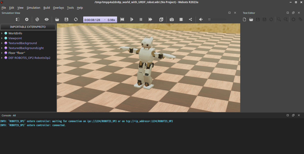
2.Webots上のロボットを動かすC++ の試作プログラムを、そのまま外部PluginのWalkingPatternGenerator.cpp に適用して、Webots上のロボットを動かした。C++ 試作プログラムの出力結果に示されている関節角度[rad]をWebots上のロボットの左脚に適用した。
以上で、逆運動学解を元にロボットを動かせた。